利用者:Pitfall99/sandbox

高次元データ（表現するのに２次元、３次元以上が必要なデータ）は解釈が難しいです。簡単に解釈するためには関心があるデータが低次元にあると仮定することです。興味があるデータが十分に低次元であれば、データを低次元に可視化することができます。

左上: 中央に長方形の穴が開いているらせん状の帯（別名スイスロール）の1000点の3Dデータセット。右上: スイスロールを２Dに伸ばしたもの。 左下と右: モジュラーデータ処理ツールキットで実装されたLLEとヘシアンLLEアルゴリズムを使用して、多様体の2D復元を行ったもの。

以下に非線形な次元削減手法の概要を説明します

Many of these non-linear dimensionality reduction methods are related to the linear methods listed below. Non-linear methods can be broadly classified into two groups: those that provide a mapping (either from the high-dimensional space to the low-dimensional embedding or vice versa), and those that just give a visualisation.

これらの非線形次元削減法の多くは、以下に列挙する線形法に関連しています。非線形手法は、マッピング（高次元空間から低次元埋め込みへのマッピング、またはその逆）を提供するものと、単に可視化を提供するものの2つのグループに大別されます。

関連する非線形な次元削減手法

• Independent component analysis (ICA).
• Principal component analysis (PCA) (also called Karhunen–Loève theorem – KLT).
• Singular value decomposition (SVD).
• Factor analysis.

Applications of NLDR

Consider a dataset represented as a matrix (or a database table), such that each row represents a set of attributes (or features or dimensions) that describe a particular instance of something. If the number of attributes is large, then the space of unique possible rows is exponentially large. Thus, the larger the dimensionality, the more difficult it becomes to sample the space. This causes many problems. Algorithms that operate on high-dimensional data tend to have a very high time complexity. Many machine learning algorithms, for example, struggle with high-dimensional data. Reducing data into fewer dimensions often makes analysis algorithms more efficient, and can help machine learning algorithms make more accurate predictions.

行列（またはデータベーステーブル）で表されるデータセットを考えてみましょう．属性の数が大きいと，一意になり得る行の空間は指数関数的に大きくなります．したがって，次元数が大きくなればなるほど，空間をサンプリングすることが難しくなります．これは多くの問題を引き起こします。高次元データ上で動作するアルゴリズムは、非常に高い時間的複雑さを持つ傾向があります。例えば、多くの機械学習アルゴリズムは、高次元データに苦戦しています。データをより少ない次元に減らすことで、多くの場合、分析アルゴリズムをより効率的にすることができ、機械学習アルゴリズムがより正確な予測を行うのに役立ちます。

Humans often have difficulty comprehending data in many dimensions. Thus, reducing data to a small number of dimensions is useful for visualization purposes.

人間は、多くの次元のデータを理解するのが難しいことが多い。そのため、データを少数の次元に縮小することは、可視化の目的で有用です。

ファイル:Nldr.jpg

Plot of the two-dimensional points that results from using a NLDR algorithm. In this case, Manifold Sculpting used to reduce the data into just two dimensions (rotation and scale).

The reduced-dimensional representations of data are often referred to as "intrinsic variables". This description implies that these are the values from which the data was produced. For example, consider a dataset that contains images of a letter 'A', which has been scaled and rotated by varying amounts. Each image has 32x32 pixels. Each image can be represented as a vector of 1024 pixel values. Each row is a sample on a two-dimensional manifold in 1024-dimensional space (a Hamming space). The intrinsic dimensionality is two, because two variables (rotation and scale) were varied in order to produce the data. Information about the shape or look of a letter 'A' is not part of the intrinsic variables because it is the same in every instance. Nonlinear dimensionality reduction will discard the correlated information (the letter 'A') and recover only the varying information (rotation and scale). The image to the right shows sample images from this dataset (to save space, not all input images are shown), and a plot of the two-dimensional points that results from using a NLDR algorithm (in this case, Manifold Sculpting was used) to reduce the data into just two dimensions.

データの低次元表現は、しばしば "固有変数 "と呼ばれています。この説明は，これらがデータが生成された値であることを意味している．例えば，文字「A」の画像を含むデータセットを考えてみましょう．各画像は32x32ピクセルである．各画像は1024ピクセルの値のベクトルとして表すことができます。各行は1024次元空間（ハミング空間）の2次元多様体上のサンプルです。データを生成するために2つの変数（回転とスケール）を変化させているため、固有の次元性は2です。文字「A」の形状や外観に関する情報は、すべてのインスタンスで同じであるため、固有の変数の一部ではありません。非線形次元削減は、相関関係のある情報（「A」の文字）を破棄し、変化する情報（回転とスケール）だけを回復します。右の画像は、このデータセットからのサンプル画像（スペースを節約するため、すべての入力画像が表示されているわけではありません）と、NLDRアルゴリズム（この場合、マニホールド・スカルプティングが使用されています）を使用してデータを2次元に縮小した結果の2次元点のプロットを示しています。

www.DeepL.com/Translator（無料版）で翻訳しました。

PCA (a linear dimensionality reduction algorithm) is used to reduce this same dataset into two dimensions, the resulting values are not so well organized.

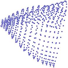
By comparison, if Principal component analysis, which is a linear dimensionality reduction algorithm, is used to reduce this same dataset into two dimensions, the resulting values are not so well organized. This demonstrates that the high-dimensional vectors (each representing a letter 'A') that sample this manifold vary in a non-linear manner.

比較すると、線形次元削減アルゴリズムである主成分分析が、この同じデータセットを2次元に削減するために使用された場合、結果として得られる値はそれほどうまく整理されていません。これは、この多様体を標本化する高次元ベクトル（それぞれが文字「A」を表す）が非線形な方法で変化することを示しています。

It should be apparent, therefore, that NLDR has several applications in the field of computer-vision. For example, consider a robot that uses a camera to navigate in a closed static environment. The images obtained by that camera can be considered to be samples on a manifold in high-dimensional space, and the intrinsic variables of that manifold will represent the robot's position and orientation. This utility is not limited to robots. Dynamical systems, a more general class of systems, which includes robots, are defined in terms of a manifold. Active research in NLDR seeks to unfold the observation manifolds associated with dynamical systems to develop techniques for modeling such systems and enable them to operate autonomously.

したがって、NLDRはコンピュータビジョンの分野でいくつかの応用があることは明らかである。例えば、カメラを使って静止した閉空間を移動するロボットを考えてみましょう。そのカメラで得られた画像は、高次元空間のマニホールド上のサンプルと考えることができ、そのマニホールドの内在変数がロボットの位置と向きを表します。この有用性はロボットに限定されるものではありません。動的システムは、ロボットを含むシステムのより一般的なクラスであり、多様体の観点から定義されます。NLDRでは、動的システムに関連した観測多様体を展開し、そのようなシステムをモデル化し、自律的に動作させる技術を開発しようとする研究が活発に行われています。

Some of the more prominent nonlinear dimensionality reduction techniques are listed below.

より著名な非線形次元削減技術のいくつかを以下に示します。

主要コンセプト

Sammon's mapping

Sammon's mapping is one of the first and most popular NLDR techniques.

Sammon's mapping は最初の非線形次元削減法である。

Approximation of a principal curve by one-dimensional SOM (a broken line with red squares, 20 nodes). The first principal component is presented by a blue straight line. Data points are the small grey circles. For PCA, the Fraction of variance unexplained in this example is 23.23%, for SOM it is 6.86%.一次元SOMによる主曲線の近似(赤四角の折れ線、20節点)。最初の主成分は青の直線で示される。データ点は小さな灰色の円。PCAの場合、この例では、説明されていない分散の割合は23.23%ですが、SOMの場合は6.86%です。

自己組織化写像（Self-organizing maps）

The self-organizing map (SOM, also called Kohonen map) and its probabilistic variant generative topographic mapping (GTM) use a point representation in the embedded space to form a latent variable model based on a non-linear mapping from the embedded space to the high-dimensional space. These techniques are related to work on density networks, which also are based around the same probabilistic model.

自己組織化写像（SOM、kohonen mapとも呼ばれる）とその確率的なバリアントである生成的地形マッピング（GMT：generative topographic mapping）は、埋め込み空間から高次元空間への非線形マッピングに基づく潜在変数モデルを形成するために、埋め込み空間の点表現を使用します。これらの技術は、同じ確率モデルに基づく密度ネットワークの研究に関連しています

Kernel principal component analysis

Perhaps the most widely used algorithm for dimensional reduction is kernel PCA. PCA begins by computing the covariance matrix of the $m\times n$ matrix $\mathbf {X}$

おそらく、次元削減のために最も広く使われているアルゴリズムは、カーネルPCAです。PCAは共分散行列を計算することから始めます。

$C={\frac {1}{m}}\sum _{i=1}^{m}{\mathbf {x} _{i}\mathbf {x} _{i}^{\mathsf {T}}}.$

It then projects the data onto the first k eigenvectors of that matrix. By comparison, KPCA begins by computing the covariance matrix of the data after being transformed into a higher-dimensional space,

そして，その行列の最初のk個の固有ベクトルにデータを投影します．これと比較して，KPCA は，高次元空間に変換された後のデータの共分散行列を計算することから始まります．

$C={\frac {1}{m}}\sum _{i=1}^{m}{\Phi (\mathbf {x} _{i})\Phi (\mathbf {x} _{i})^{\mathsf {T}}}.$

It then projects the transformed data onto the first k eigenvectors of that matrix, just like PCA. It uses the kernel trick to factor away much of the computation, such that the entire process can be performed without actually computing $\Phi (\mathbf {x} )$. Of course $\Phi$ must be chosen such that it has a known corresponding kernel. Unfortunately, it is not trivial to find a good kernel for a given problem, so KPCA does not yield good results with some problems when using standard kernels. For example, it is known to perform poorly with these kernels on the Swiss roll manifold. However, one can view certain other methods that perform well in such settings (e.g., Laplacian Eigenmaps, LLE) as special cases of kernel PCA by constructing a data-dependent kernel matrix.

そして，PCAと同様に，変換されたデータをその行列の最初のk個の固有ベクトルに投影します．これは，カーネルのトリックを利用して，計算の多くを因数分解することで，実際には

KPCA has an internal model, so it can be used to map points onto its embedding that were not available at training time.

Principal curves and manifolds

Application of principal curves: Nonlinear quality of life index. Points represent data of the UN 171 countries in 4-dimensional space formed by the values of 4 indicators: gross product per capita, life expectancy, infant mortality, tuberculosis incidence. Different forms and colors correspond to various geographical locations. Red bold line represents the principal curve, approximating the dataset. This principal curve was produced by the method of elastic map. Software is available for free non-commercial use.

Principal curves and manifolds give the natural geometric framework for nonlinear dimensionality reduction and extend the geometric interpretation of PCA by explicitly constructing an embedded manifold, and by encoding using standard geometric projection onto the manifold. This approach was proposed by Trevor Hastie in his thesis (1984) and developed further by many authors. How to define the "simplicity" of the manifold is problem-dependent, however, it is commonly measured by the intrinsic dimensionality and/or the smoothness of the manifold. Usually, the principal manifold is defined as a solution to an optimization problem. The objective function includes a quality of data approximation and some penalty terms for the bending of the manifold. The popular initial approximations are generated by linear PCA and Kohonen's SOM.

主曲線と多様体は、非線形次元削減のための自然な幾何学的枠組みを与え、明示的に埋め込まれた多様体を構築し、その多様体への標準的な幾何学的投影を用いて符号化することで、PCAの幾何学的解釈を拡張します。このアプローチは、Trevor Hastieによって彼の論文(1984)で提案され、多くの著者によってさらに発展しました。マニホールドの「単純さ」をどのように定義するかは問題に依存しますが、一般的には内在的な次元性やマニホールドの滑らかさによって測定されます。通常、主多様体は最適化問題の解として定義されます。目的関数には、データの品質近似と、マニホールドの曲がりに対するいくつかのペナルティ項が含まれています。一般的な初期近似は、線形PCAとKohonenのSOMによって生成されます。

Laplacian eigenmaps

「Manifold regularization」も参照

Laplacian Eigenmaps uses spectral techniques to perform dimensionality reduction. This technique relies on the basic assumption that the data lies in a low-dimensional manifold in a high-dimensional space. This algorithm cannot embed out-of-sample points, but techniques based on Reproducing kernel Hilbert space regularization exist for adding this capability. Such techniques can be applied to other nonlinear dimensionality reduction algorithms as well.

ラプラシアン固有マップは、次元削減を実行するためにスペクトル技術を使用します。この手法は、データが高次元空間の低次元多様体にあるという基本的な仮定に依存しています。このアルゴリズムは、サンプル外の点を埋め込むことはできませんが、この機能を追加するために、再現カーネル・ヒルベルト空間正則化に基づく技術が存在します。このような技術は、他の非線形次元削減アルゴリズムにも適用することができます。

Traditional techniques like principal component analysis do not consider the intrinsic geometry of the data. Laplacian eigenmaps builds a graph from neighborhood information of the data set. Each data point serves as a node on the graph and connectivity between nodes is governed by the proximity of neighboring points (using e.g. the k-nearest neighbor algorithm). The graph thus generated can be considered as a discrete approximation of the low-dimensional manifold in the high-dimensional space. Minimization of a cost function based on the graph ensures that points close to each other on the manifold are mapped close to each other in the low-dimensional space, preserving local distances. The eigenfunctions of the Laplace–Beltrami operator on the manifold serve as the embedding dimensions, since under mild conditions this operator has a countable spectrum that is a basis for square integrable functions on the manifold (compare to Fourier series on the unit circle manifold). Attempts to place Laplacian eigenmaps on solid theoretical ground have met with some success, as under certain nonrestrictive assumptions, the graph Laplacian matrix has been shown to converge to the Laplace–Beltrami operator as the number of points goes to infinity.

主成分分析のような従来の手法では、データの本質的な形状を考慮していません。ラプラシアン固有マップは、データセットの近傍情報からグラフを構築します。各データ点はグラフ上のノードとして機能し、ノード間の接続性は隣接点の近さによって制御されます（例：k-nearest neighborアルゴリズムを使用）。このようにして生成されたグラフは、高次元空間における低次元多様体の離散的な近似と考えることができます。グラフに基づくコスト関数の最小化は、局所的な距離を維持しながら、多様体上で互いに近い点が低次元空間内で互いに近い位置に写されることを保証します。マニホールド上のラプラス-ベルトラミ演算子の固有関数が埋め込み次元として機能します。軽度の条件では、この演算子は、（単位円マニホールド上のフーリエ級数と比較して）マニホールド上の正方可積分関数の基礎となるカウント可能なスペクトルを持っているためです。ラプラシアンの固有マップを理論的な根拠に基づいて配置しようとする試みは、ある種の非制限的な仮定の下で、グラフのラプラシアン行列が点の数が無限大になるにつれてラプラス-ベルトラミ演算子に収束することが示されているため、いくつかの成功を収めています。

In classification applications, low dimension manifolds can be used to model data classes which can be defined from sets of observed instances. Each observed instance can be described by two independent factors termed ’content’ and ’style’, where ’content’ is the invariant factor related to the essence of the class and ’style’ expresses variations in that class between instances. Unfortunately, Laplacian Eigenmaps may fail to produce a coherent representation of a class of interest when training data consist of instances varying significantly in terms of style. In the case of classes which are represented by multivariate sequences, Structural Laplacian Eigenmaps has been proposed to overcome this issue by adding additional constraints within the Laplacian Eigenmaps neighborhood information graph to better reflect the intrinsic structure of the class. More specifically, the graph is used to encode both the sequential structure of the multivariate sequences and, to minimise stylistic variations, proximity between data points of different sequences or even within a sequence, if it contains repetitions. Using dynamic time warping, proximity is detected by finding correspondences between and within sections of the multivariate sequences that exhibit high similarity. Experiments conducted on vision-based activity recognition, object orientation classification and human 3D pose recovery applications have demonstrate the added value of Structural Laplacian Eigenmaps when dealing with multivariate sequence data. An extension of Structural Laplacian Eigenmaps, Generalized Laplacian Eigenmaps led to the generation of manifolds where one of the dimensions specifically represents variations in style. This has proved particularly valuable in applications such as tracking of the human articulated body and silhouette extraction.

Isomap

Isomap is a combination of the Floyd–Warshall algorithm with classic Multidimensional Scaling. Classic Multidimensional Scaling (MDS) takes a matrix of pair-wise distances between all points and computes a position for each point. Isomap assumes that the pair-wise distances are only known between neighboring points, and uses the Floyd–Warshall algorithm to compute the pair-wise distances between all other points. This effectively estimates the full matrix of pair-wise geodesic distances between all of the points. Isomap then uses classic MDS to compute the reduced-dimensional positions of all the points. Landmark-Isomap is a variant of this algorithm that uses landmarks to increase speed, at the cost of some accuracy.

In manifold learning, the input data is assumed to be sampled from a low dimensional manifold that is embedded inside of a higher-dimensional vector space. The main intuition behind MVU is to exploit the local linearity of manifolds and create a mapping that preserves local neighbourhoods at every point of the underlying manifold.

Locally-linear embedding

Locally-Linear Embedding (LLE) was presented at approximately the same time as Isomap. It has several advantages over Isomap, including faster optimization when implemented to take advantage of sparse matrix algorithms, and better results with many problems. LLE also begins by finding a set of the nearest neighbors of each point. It then computes a set of weights for each point that best describes the point as a linear combination of its neighbors. Finally, it uses an eigenvector-based optimization technique to find the low-dimensional embedding of points, such that each point is still described with the same linear combination of its neighbors. LLE tends to handle non-uniform sample densities poorly because there is no fixed unit to prevent the weights from drifting as various regions differ in sample densities. LLE has no internal model.

LLE computes the barycentric coordinates of a point X_i based on its neighbors X_j. The original point is reconstructed by a linear combination, given by the weight matrix W_ij, of its neighbors. The reconstruction error is given by the cost function E(W).

$E(W)=\sum _{i}|{\mathbf {X} _{i}-\sum _{j}{\mathbf {W} _{ij}\mathbf {X} _{j}}|}^{\mathsf {2}}$

The weights W_ij refer to the amount of contribution the point X_j has while reconstructing the point X_i. The cost function is minimized under two constraints: (a) Each data point X_i is reconstructed only from its neighbors, thus enforcing W_ij to be zero if point X_j is not a neighbor of the point X_i and (b) The sum of every row of the weight matrix equals 1.

$\sum _{j}{\mathbf {W} _{ij}}=1$

The original data points are collected in a D dimensional space and the goal of the algorithm is to reduce the dimensionality to d such that D >> d. The same weights W_ij that reconstructs the ith data point in the D dimensional space will be used to reconstruct the same point in the lower d dimensional space. A neighborhood preserving map is created based on this idea. Each point X_i in the D dimensional space is mapped onto a point Y_i in the d dimensional space by minimizing the cost function

$C(Y)=\sum _{i}|{\mathbf {Y} _{i}-\sum _{j}{\mathbf {W} _{ij}\mathbf {Y} _{j}}|}^{\mathsf {2}}$

In this cost function, unlike the previous one, the weights W_ij are kept fixed and the minimization is done on the points Y_i to optimize the coordinates. This minimization problem can be solved by solving a sparse N X N eigen value problem (N being the number of data points), whose bottom d nonzero eigen vectors provide an orthogonal set of coordinates. Generally the data points are reconstructed from K nearest neighbors, as measured by Euclidean distance. For such an implementation the algorithm has only one free parameter K, which can be chosen by cross validation.

Hessian Locally-Linear Embedding (Hessian LLE)

Like LLE, Hessian LLE is also based on sparse matrix techniques. It tends to yield results of a much higher quality than LLE. Unfortunately, it has a very costly computational complexity, so it is not well-suited for heavily sampled manifolds. It has no internal model.

Modified Locally-Linear Embedding (MLLE)

Modified LLE (MLLE) is another LLE variant which uses multiple weights in each neighborhood to address the local weight matrix conditioning problem which leads to distortions in LLE maps. Loosely speaking the multiple weights are the local orthogonal projection of the original weights produced by LLE. The creators of this regularised variant are also the authors of Local Tangent Space Alignment (LTSA), which is implicit in the MLLE formulation when realising that the global optimisation of the orthogonal projections of each weight vector, in-essence, aligns the local tangent spaces of every data point. The theoretical and empirical implications from the correct application of this algorithm are far-reaching.

Local tangent space alignment

詳細は「Local tangent space alignment」を参照

LTSA is based on the intuition that when a manifold is correctly unfolded, all of the tangent hyperplanes to the manifold will become aligned. It begins by computing the k-nearest neighbors of every point. It computes the tangent space at every point by computing the d-first principal components in each local neighborhood. It then optimizes to find an embedding that aligns the tangent spaces.

Maximum variance unfolding

Maximum Variance Unfolding, Isomap and Locally Linear Embedding share a common intuition relying on the notion that if a manifold is properly unfolded, then variance over the points is maximized. Its initial step, like Isomap and Locally Linear Embedding, is finding the k-nearest neighbors of every point. It then seeks to solve the problem of maximizing the distance between all non-neighboring points, constrained such that the distances between neighboring points are preserved. The primary contribution of this algorithm is a technique for casting this problem as a semidefinite programming problem. Unfortunately, semidefinite programming solvers have a high computational cost. Like Locally Linear Embedding, it has no internal model.

Autoencoders

An autoencoder is a feed-forward neural network which is trained to approximate the identity function. That is, it is trained to map from a vector of values to the same vector. When used for dimensionality reduction purposes, one of the hidden layers in the network is limited to contain only a small number of network units. Thus, the network must learn to encode the vector into a small number of dimensions and then decode it back into the original space. Thus, the first half of the network is a model which maps from high to low-dimensional space, and the second half maps from low to high-dimensional space. Although the idea of autoencoders is quite old, training of deep autoencoders has only recently become possible through the use of restricted Boltzmann machines and stacked denoising autoencoders. Related to autoencoders is the NeuroScale algorithm, which uses stress functions inspired by multidimensional scaling and Sammon mappings (see above) to learn a non-linear mapping from the high-dimensional to the embedded space. The mappings in NeuroScale are based on radial basis function networks. Another usage of a neural network for dimensionality reduction is to make it learn the tangent planes in the data.

Gaussian process latent variable models

Gaussian process latent variable models (GPLVM) are probabilistic dimensionality reduction methods that use Gaussian Processes (GPs) to find a lower dimensional non-linear embedding of high dimensional data. They are an extension of the Probabilistic formulation of PCA. The model is defined probabilistically and the latent variables are then marginalized and parameters are obtained by maximizing the likelihood. Like kernel PCA they use a kernel function to form a non linear mapping (in the form of a Gaussian process). However, in the GPLVM the mapping is from the embedded(latent) space to the data space (like density networks and GTM) whereas in kernel PCA it is in the opposite direction. It was originally proposed for visualization of high dimensional data but has been extended to construct a shared manifold model between two observation spaces. GPLVM and its many variants have been proposed specially for human motion modeling, e.g., back constrained GPLVM, GP dynamic model (GPDM), balanced GPDM (B-GPDM) and topologically constrained GPDM. To capture the coupling effect of the pose and gait manifolds in the gait analysis, a multi-layer joint gait-pose manifolds was proposed.

t-distributed stochastic neighbor embedding

t-distributed stochastic neighbor embedding (t-SNE) is widely used. It is one of a family of stochastic neighbor embedding methods. The algorithm computes the probability that pairs of datapoints in the high-dimensional space are related, and then chooses low-dimensional embeddings which produce a similar distribution.

Other algorithms

Relational perspective map

Relational perspective map is a multidimensional scaling algorithm. The algorithm finds a configuration of data points on a manifold by simulating a multi-particle dynamic system on a closed manifold, where data points are mapped to particles and distances (or dissimilarity) between data points represent a repulsive force. As the manifold gradually grows in size the multi-particle system cools down gradually and converges to a configuration that reflects the distance information of the data points.

Relational perspective map was inspired by a physical model in which positively charged particles move freely on the surface of a ball. Guided by the Coulomb force between particles, the minimal energy configuration of the particles will reflect the strength of repulsive forces between the particles.

The Relational perspective map was introduced in. The algorithm firstly used the flat torus as the image manifold, then it has been extended (in the software VisuMap to use other types of closed manifolds, like the sphere, projective space, and Klein bottle, as image manifolds.

Contagion maps

Contagion maps use multiple contagions on a network to map the nodes as a point cloud. In the case of the Global cascades model the speed of the spread can be adjusted with the threshold parameter $t\in [0,1]$. For $t=0$ the contagion map is equivalent to the Isomap algorithm.

Curvilinear component analysis

Curvilinear component analysis (CCA) looks for the configuration of points in the output space that preserves original distances as much as possible while focusing on small distances in the output space (conversely to Sammon's mapping which focus on small distances in original space).

It should be noticed that CCA, as an iterative learning algorithm, actually starts with focus on large distances (like the Sammon algorithm), then gradually change focus to small distances. The small distance information will overwrite the large distance information, if compromises between the two have to be made.

The stress function of CCA is related to a sum of right Bregman divergences.

Curvilinear distance analysis

CDA trains a self-organizing neural network to fit the manifold and seeks to preserve geodesic distances in its embedding. It is based on Curvilinear Component Analysis (which extended Sammon's mapping), but uses geodesic distances instead.

Diffeomorphic dimensionality reduction

Diffeomorphic Dimensionality Reduction or Diffeomap learns a smooth diffeomorphic mapping which transports the data onto a lower-dimensional linear subspace. The methods solves for a smooth time indexed vector field such that flows along the field which start at the data points will end at a lower-dimensional linear subspace, thereby attempting to preserve pairwise differences under both the forward and inverse mapping.

Manifold alignment

Manifold alignment takes advantage of the assumption that disparate data sets produced by similar generating processes will share a similar underlying manifold representation. By learning projections from each original space to the shared manifold, correspondences are recovered and knowledge from one domain can be transferred to another. Most manifold alignment techniques consider only two data sets, but the concept extends to arbitrarily many initial data sets.

Diffusion maps

Diffusion maps leverages the relationship between heat diffusion and a random walk (Markov Chain); an analogy is drawn between the diffusion operator on a manifold and a Markov transition matrix operating on functions defined on the graph whose nodes were sampled from the manifold. In particular, let a data set be represented by $\mathbf {X} =[x_{1},x_{2},\ldots ,x_{n}]\in \Omega \subset \mathbf {R^{D}}$. The underlying assumption of diffusion map is that the high-dimensional data lies on a low-dimensional manifold of dimension $\mathbf {d}$. Let X represent the data set and $\mu$ represent the distribution of the data points on X. Further, define a kernel which represents some notion of affinity of the points in X. The kernel ${\mathit {k}}$ has the following properties

$k(x,y)=k(y,x),\,$

k is symmetric

$k(x,y)\geq 0\qquad \forall x,y,k$

k is positivity preserving

Thus one can think of the individual data points as the nodes of a graph and the kernel k as defining some sort of affinity on that graph. The graph is symmetric by construction since the kernel is symmetric. It is easy to see here that from the tuple (X,k) one can construct a reversible Markov Chain. This technique is common to a variety of fields and is known as the graph Laplacian.

For example, the graph K = (X,E) can be constructed using a Gaussian kernel.

$K_{ij}={\begin{cases}e^{-\|x_{i}-x_{j}\|_{2}^{2}/\sigma ^{2}}&{\text{if }}x_{i}\sim x_{j}\\0&{\text{otherwise}}\end{cases}}$

In the above equation, $x_{i}\sim x_{j}$ denotes that $x_{i}$ is a nearest neighbor of $x_{j}$. Properly, Geodesic distance should be used to actually measure distances on the manifold. Since the exact structure of the manifold is not available, for the nearest neighbors the geodesic distance is approximated by euclidean distance. The choice $\sigma$ modulates our notion of proximity in the sense that if $\|x_{i}-x_{j}\|_{2}\gg \sigma$ then $K_{ij}=0$ and if $\|x_{i}-x_{j}\|_{2}\ll \sigma$ then $K_{ij}=1$. The former means that very little diffusion has taken place while the latter implies that the diffusion process is nearly complete. Different strategies to choose $\sigma$ can be found in.

In order to faithfully represent a Markov matrix, $K$ must be normalized by the corresponding degree matrix $D$:

$P=D^{-1}K.\,$

$P$ now represents a Markov chain. $P(x_{i},x_{j})$ is the probability of transitioning from $x_{i}$ to $x_{j}$ in one time step. Similarly the probability of transitioning from $x_{i}$ to $x_{j}$ in t time steps is given by $P^{t}(x_{i},x_{j})$. Here $P^{t}$ is the matrix $P$ multiplied by itself t times.

The Markov matrix $P$ constitutes some notion of local geometry of the data set X. The major difference between diffusion maps and principal component analysis is that only local features of the data are considered in diffusion maps as opposed to taking correlations of the entire data set.

$K$ defines a random walk on the data set which means that the kernel captures some local geometry of data set. The Markov chain defines fast and slow directions of propagation through the kernel values. As the walk propagates forward in time, the local geometry information aggregates in the same way as local transitions (defined by differential equations) of the dynamical system. The metaphor of diffusion arises from the definition of a family diffusion distance {$D_{t}$}$_{t\in N}$

$D_{t}^{2}(x,y)=||p_{t}(x,\cdot )-p_{t}(y,\cdot )||^{2}$

For fixed t, $D_{t}$ defines a distance between any two points of the data set based on path connectivity: the value of $D_{t}(x,y)$ will be smaller the more paths that connect x to y and vice versa. Because the quantity $D_{t}(x,y)$ involves a sum over of all paths of length t, $D_{t}$ is much more robust to noise in the data than geodesic distance. $D_{t}$ takes into account all the relation between points x and y while calculating the distance and serves as a better notion of proximity than just Euclidean distance or even geodesic distance.

Local multidimensional scaling

Local Multidimensional Scaling performs multidimensional scaling in local regions, and then uses convex optimization to fit all the pieces together.

Nonlinear PCA

Nonlinear PCA (NLPCA) uses backpropagation to train a multi-layer perceptron (MLP) to fit to a manifold. Unlike typical MLP training, which only updates the weights, NLPCA updates both the weights and the inputs. That is, both the weights and inputs are treated as latent values. After training, the latent inputs are a low-dimensional representation of the observed vectors, and the MLP maps from that low-dimensional representation to the high-dimensional observation space.

Data-driven high-dimensional scaling

Data-Driven High Dimensional Scaling (DD-HDS) is closely related to Sammon's mapping and curvilinear component analysis except that (1) it simultaneously penalizes false neighborhoods and tears by focusing on small distances in both original and output space, and that (2) it accounts for concentration of measure phenomenon by adapting the weighting function to the distance distribution.

Manifold sculpting

Manifold Sculpting uses graduated optimization to find an embedding. Like other algorithms, it computes the k-nearest neighbors and tries to seek an embedding that preserves relationships in local neighborhoods. It slowly scales variance out of higher dimensions, while simultaneously adjusting points in lower dimensions to preserve those relationships. If the rate of scaling is small, it can find very precise embeddings. It boasts higher empirical accuracy than other algorithms with several problems. It can also be used to refine the results from other manifold learning algorithms. It struggles to unfold some manifolds, however, unless a very slow scaling rate is used. It has no model.

RankVisu

RankVisu is designed to preserve rank of neighborhood rather than distance. RankVisu is especially useful on difficult tasks (when the preservation of distance cannot be achieved satisfyingly). Indeed, the rank of neighborhood is less informative than distance (ranks can be deduced from distances but distances cannot be deduced from ranks) and its preservation is thus easier.

Topologically constrained isometric embedding

Topologically Constrained Isometric Embedding (TCIE) is an algorithm based on approximating geodesic distances after filtering geodesics inconsistent with the Euclidean metric. Aimed at correcting the distortions caused when Isomap is used to map intrinsically non-convex data, TCIE uses weight least-squares MDS in order to obtain a more accurate mapping. The TCIE algorithm first detects possible boundary points in the data, and during computation of the geodesic length marks inconsistent geodesics, to be given a small weight in the weighted Stress majorization that follows.

Uniform manifold approximation and projection

Uniform manifold approximation and projection (UMAP) is a nonlinear dimensionality reduction technique. Visually, it is similar to t-SNE, but it assumes that the data is uniformly distributed on a locally connected Riemannian manifold and that the Riemannian metric is locally constant or approximately locally constant.

Methods based on proximity matrices

A method based on proximity matrices is one where the data is presented to the algorithm in the form of a similarity matrix or a distance matrix. These methods all fall under the broader class of metric multidimensional scaling. The variations tend to be differences in how the proximity data is computed; for example, Isomap, locally linear embeddings, maximum variance unfolding, and Sammon mapping (which is not in fact a mapping) are examples of metric multidimensional scaling methods.

See also

• Discriminant analysis
• Elastic map
• Feature learning
• Growing self-organizing map (GSOM)
• Self-organizing map (SOM)
• Taken's theorem
• Whitney embedding theorem

External links

• Isomap
• Generative Topographic Mapping
• Mike Tipping's Thesis
• Gaussian Process Latent Variable Model
• Locally Linear Embedding
• Relational Perspective Map
• Waffles is an open source C++ library containing implementations of LLE, Manifold Sculpting, and some other manifold learning algorithms.
• DD-HDS homepage
• RankVisu homepage
• Short review of Diffusion Maps
• Nonlinear PCA by autoencoder neural networks

References

[編集]- ^ Lawrence, Neil D (2012). “A unifying probabilistic perspective for spectral dimensionality reduction: insights and new models”. Journal of Machine Learning Research 13 (May): 1609–1638. arXiv:1010.4830. Bibcode: 2010arXiv1010.4830L.
- ^ John A. Lee, Michel Verleysen, Nonlinear Dimensionality Reduction, Springer, 2007.
- ^ Gashler, M. and Martinez, T., Temporal Nonlinear Dimensionality Reduction, In Proceedings of the International Joint Conference on Neural Networks IJCNN'11, pp. 1959–1966, 2011
- ^ The illustration is prepared using free software: E.M. Mirkes, Principal Component Analysis and Self-Organizing Maps: applet. University of Leicester, 2011
- ^ Yin, Hujun; Learning Nonlinear Principal Manifolds by Self-Organising Maps, in A.N. Gorban, B. Kégl, D.C. Wunsch, and A. Zinovyev (Eds.), Principal Manifolds for Data Visualization and Dimension Reduction, Lecture Notes in Computer Science and Engineering (LNCSE), vol. 58, Berlin, Germany: Springer, 2007, Ch. 3, pp. 68-95. ISBN 978-3-540-73749-0
- ^ B. Schölkopf, A. Smola, K.-R. Müller, Nonlinear Component Analysis as a Kernel Eigenvalue Problem. Neural Computation 10(5):1299-1319, 1998, MIT Press Cambridge, MA, USA, doi:10.1162/089976698300017467
- ^ Jihun Ham, Daniel D. Lee, Sebastian Mika, Bernhard Schölkopf. A kernel view of the dimensionality reduction of manifolds. Proceedings of the 21st International Conference on Machine Learning, Banff, Canada, 2004. doi:10.1145/1015330.1015417
- ^ Gorban, A. N.; Zinovyev, A. (2010). “Principal manifolds and graphs in practice: from molecular biology to dynamical systems”. International Journal of Neural Systems 20 (3): 219–232. arXiv:1001.1122. doi:10.1142/S0129065710002383. PMID 20556849.
- ^ A. Zinovyev, ViDaExpert - Multidimensional Data Visualization Tool (free for non-commercial use). Institut Curie, Paris.
- ^ A. Zinovyev, ViDaExpert overview, IHES (Institut des Hautes Études Scientifiques), Bures-Sur-Yvette, Île-de-France.
- ^ Hastie, T. (November 1984). Principal Curves and Surfaces (PDF) (PhD Dissertation). Stanford Linear Accelerator Center, Stanford University.
- ^ Gorban, A. N.; Kégl, B.; Wunsch, D. C. et al., eds (2007). Principal Manifolds for Data Visualisation and Dimension Reduction. Lecture Notes in Computer Science and Engineering (LNCSE). Vol. 58. Berlin – Heidelberg – New York: Springer. ISBN 978-3-540-73749-0
- ^ Belkin, Mikhail; Niyogi, Partha (2001). “Laplacian Eigenmaps and Spectral Techniques for Embedding and Clustering”. Advances in Neural Information Processing Systems (MIT Press) 14: 586–691.
- ^ a b Belkin, Mikhail (August 2003). Problems of Learning on Manifolds (PhD Thesis). Department of Mathematics, The University of Chicago. Matlab code for Laplacian Eigenmaps can be found in algorithms at Ohio-state.edu
- ^ Bengio, Yoshua et al. (2004). “Out-of-Sample Extensions for LLE, Isomap, MDS, Eigenmaps, and Spectral Clustering”. Advances in Neural Information Processing Systems
- ^ Tenenbaum, J.; Freeman, W. (2000). “Separating style and content with bilinear models”. Neural Computation 12 (6): 1247–1283. doi:10.1162/089976600300015349. PMID 10935711.
- ^ Lewandowski, M.; Martinez-del Rincon, J.; Makris, D.; Nebel, J.-C. (2010). “Temporal extension of laplacian eigenmaps for unsupervised dimensionality reduction of time series”. Proceedings of the International Conference on Pattern Recognition (ICPR)
- ^ a b Lewandowski, M.; Makris, D.; Velastin, S. A.; Nebel, J.-C. (2014). “Structural Laplacian Eigenmaps for Modeling Sets of Multivariate Sequences”. IEEE Transactions on Cybernetics 44 (6): 936–949. doi:10.1109/TCYB.2013.2277664. PMID 24144690.
- ^ Martinez-del-Rincon, J.; Lewandowski, M.; Nebel, J.-C.; Makris, D. (2014). “Generalized Laplacian Eigenmaps for Modeling and Tracking Human Motions”. IEEE Transactions on Cybernetics 44 (9): 1646–1660. doi:10.1109/TCYB.2013.2291497. PMID 25137692.
- ^ J. B. Tenenbaum, V. de Silva, J. C. Langford, A Global Geometric Framework for Nonlinear Dimensionality Reduction, Science 290, (2000), 2319–2323.
- ^ S. T. Roweis and L. K. Saul, Nonlinear Dimensionality Reduction by Locally Linear Embedding, Science Vol 290, 22 December 2000, 2323–2326.
- ^ Donoho, D.; Grimes, C. (2003). “Hessian eigenmaps: Locally linear embedding techniques for high-dimensional data”. Proc Natl Acad Sci U S A 100 (10): 5591–5596. doi:10.1073/pnas.1031596100. PMC 156245. PMID 16576753.
- ^ Z. Zhang and J. Wang, "MLLE: Modified Locally Linear Embedding Using Multiple Weights" http://citeseerx.ist.psu.edu/viewdoc/summary?doi=10.1.1.70.382
- ^ “Locally Linear Embedding and fMRI feature selection in psychiatric classification”. IEEE Journal of Translational Engineering in Health and Medicine 7: 1–11. (2019). arXiv:1908.06319. doi:10.1109/JTEHM.2019.2936348. PMC 6726465. PMID 31497410.
- ^ Zhang, Zhenyue; Hongyuan Zha (2005). “Principal Manifolds and Nonlinear Dimension Reduction via Local Tangent Space Alignment”. SIAM Journal on Scientific Computing 26 (1): 313–338. doi:10.1137/s1064827502419154.
- ^ Bengio, Yoshua; Monperrus, Martin; Larochelle, Hugo (October 2006). “Nonlocal Estimation of Manifold Structure”. Neural Computation 18 (10): 2509–2528. doi:10.1162/neco.2006.18.10.2509. ISSN 0899-7667. PMID 16907635.
- ^ N. Lawrence, Probabilistic Non-linear Principal Component Analysis with Gaussian Process Latent Variable Models, Journal of Machine Learning Research 6(Nov):1783–1816, 2005.
- ^ M. Ding, G. Fan, Multilayer Joint Gait-Pose Manifolds for Human Gait Motion Modeling, IEEE Transactions on Cybernetics, Volume: 45, Issue: 11, Nov 2015.
- ^ van der Maaten, L.J.P.; Hinton, G.E. (Nov 2008). “Visualizing High-Dimensional Data Using t-SNE”. Journal of Machine Learning Research 9: 2579–2605.
- ^ James X. Li, Visualizing high-dimensional data with relational perspective map, Information Visualization (2004) 3, 49–59
- ^ Taylor, D.; Klimm, F.; Harrington, H. A.; Kramár, M.; Mischaikow, K.; Porter, M. A.; Mucha, P. J. (2015). “Topological data analysis of contagion maps for examining spreading processes on networks”. Nature Communications 6: 7723. doi:10.1038/ncomms8723. PMC 4566922. PMID 26194875.
- ^ a b Demartines, P.; Hérault, J. (1997). “Curvilinear Component Analysis: A Self-Organizing Neural Network for Nonlinear Mapping of Data Sets”. IEEE Transactions on Neural Networks 8 (1): 148–154. doi:10.1109/72.554199. PMID 18255618.
- ^ Sun, Jigang; Crowe, Malcolm; Fyfe, Colin (2010). “Curvilinear component analysis and Bregman divergences”. European Symposium on Artificial Neural Networks (Esann). d-side publications. pp. 81–86
- ^ Christian Walder and Bernhard Schölkopf, Diffeomorphic Dimensionality Reduction, Advances in Neural Information Processing Systems 22, 2009, pp. 1713–1720, MIT Press
- ^ Wang, Chang; Mahadevan, Sridhar (July 2008). Manifold Alignment using Procrustes Analysis (PDF). The 25th International Conference on Machine Learning. pp. 1120–1127.
- ^ Lafon, Stephane (May 2004). Diffusion Maps and Geometric Harmonics (PhD Thesis). Yale University.
- ^ a b Coifman, Ronald R.; Lafon, Stephane (19 June 2006). “Diffusion Maps”. Science.
- ^ Bah, B. (2008). Diffusion Maps: Applications and Analysis (Masters Thesis). University of Oxford.
- ^ Venna, J.; Kaski, S. (2006). “Local multidimensional scaling”. Neural Networks 19 (6–7): 889–899. doi:10.1016/j.neunet.2006.05.014. PMID 16787737.
- ^ Scholz, M.; Kaplan, F.; Guy, C. L.; Kopka, J.; Selbig, J. (2005). “Non-linear PCA: a missing data approach”. Bioinformatics (Oxford University Press) 21 (20): 3887–3895. doi:10.1093/bioinformatics/bti634. PMID 16109748.
- ^ S. Lespinats, M. Verleysen, A. Giron, B. Fertil, DD-HDS: a tool for visualization and exploration of high-dimensional data, IEEE Transactions on Neural Networks 18 (5) (2007) 1265–1279.
- ^ Gashler, M. and Ventura, D. and Martinez, T., Iterative Non-linear Dimensionality Reduction with Manifold Sculpting, In Platt, J.C. and Koller, D. and Singer, Y. and Roweis, S., editor, Advances in Neural Information Processing Systems 20, pp. 513–520, MIT Press, Cambridge, MA, 2008
- ^ Lespinats S., Fertil B., Villemain P. and Herault J., Rankvisu: Mapping from the neighbourhood network, Neurocomputing, vol. 72 (13–15), pp. 2964–2978, 2009.
- ^ Rosman G., Bronstein M. M., Bronstein A. M. and Kimmel R., Nonlinear Dimensionality Reduction by Topologically Constrained Isometric Embedding, International Journal of Computer Vision, Volume 89, Number 1, 56–68, 2010
- ^ McInnes, Leland; Healy, John; Melville, James (2018年12月7日). “Uniform manifold approximation and projection for dimension reduction”
- ^ “UMAP: Uniform Manifold Approximation and Projection for Dimension Reduction — umap 0.3 documentation”. umap-learn.readthedocs.io. 2019年5月4日閲覧。